Knuth's die
This case study uses SCOOP to model a die by means of one coin, as presented by Donald Knuth. Combining forces with MRMC, we compute the probabilities of each of the sides of the die.The setting
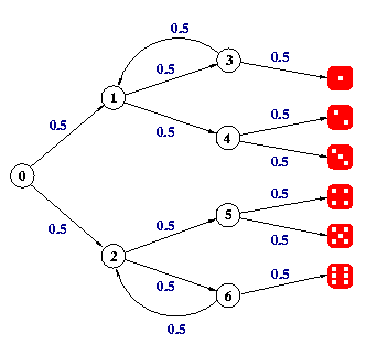
Suppose you want to play a game that necessitates a die, but you only possess a coin. It turns out that it is possible to devise an algorithm that, based on throwing the coin several times, simulates the throwing of a die. The algorithm can be visualised as follows (taken from www.prismmodelchecker.org):
Each state in this model has two outgoing edges: the upper one represents heads, the lower one represents tails. If, for instance, we throw heads heads heads tails tails, we end up throwing the number 3. Clearly, this algorithm terminates with probability 1, although it could take a while. We can use SCOOP to model this algorithm as a DTMC, and use MRMC to compute the probabilities of the different sides of the die.
The SCOOP model
To model this algorithm in SCOOP, we introduce a few processes. First of all, we let X be the initial process:X = throw.psum(1/2 -> A[] ++ 1/2 -> B[])
X throws the coin, and goes to either A or B with probability 1/2.
Those two processes provide the functionality to throw 1, 2 or 3, and 4, 5 or 6, respectively, according to the picture above.
A = throw.psum(
1/2 -> throw.psum(1/2 -> Z[1] ++ 1/2 -> Z[2])
++ 1/2 -> throw.psum(1/2 -> Z[3] ++ 1/2 -> A[]))
B = throw.psum(
1/2 -> throw.psum(1/2 -> Z[4] ++ 1/2 -> Z[5])
++ 1/2 -> throw.psum(1/2 -> Z[6] ++ 1/2 -> B[]))
When a number has been chosen, we go to the Z process. That process just keeps
repeating the chosen number:
type Die = {1..6}
Z(j:Die)= chose(j).Z[j]
Finally, the model has to be initiated:
init X
The complete model is incorporated in the web-based version of SCOOP, and can
also be found here.
Analysing the model
We use SCOOP to generate the state space of this model, and MRMC to compute the relevant probabilities. The state space is generated as follows:- scoop -aut -cadp -dtmc < knuth.prcrl > knuth.aut
- javac -classpath . AUTtoTRA.java
- java -classpath . AUTtoTRA knuth.aut
P {>= 0 } [tt U chose(1)]
$RESULT[1]
A file that contains these commands for each of the sides of a die (plus some additional commands to switch off debug information) can be found here.
It can be applied as follows:
- mrmc dtmc knuth.aut.tra knuth.aut.lab < knuth.mrmc
$RESULT[1] = 0.1666665
$RESULT[1] = 0.1666665
$RESULT[1] = 0.1666665
$RESULT[1] = 0.1666665
$RESULT[1] = 0.1666665
$RESULT[1] = 0.1666665
Apparently, the simulation indeed works as expected.
